
In the previous post I have been talking about multiple linear regression, preparing the data and model predictions.
Now we can build the optimal model using backward elimination. But why the model we built so far is not optimal? Because so far we have been using all independent variables. Some of them are highly statistically significant, which means that they have a big impact on the dependent variable “Profit”, but others are not statistically significant – they have little or no impact on the dependent variable. That means that we can remove variables that are not statistically significant from the model and still get good predictions. The goal is to find the team of independent variables where each of the variable is highly statistically significant and highly affects the dependent variable.
To accomplish this we are going to use backward elimination using the library statsmodels. To be able to use this library first we need to do a small change. Let us recall how the multiple linear regression formula looked like

Next to the coefficient 

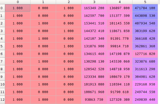
import statsmodels.formula.api as sm
x = np.append(arr = np.ones((50, 1)).astype(int), values = x, axis = 1)
In the code snippet above, we appended 50 rows of ones to the matrix
The backward elimination algorithm that we will follow is this:
- Select a significance level to stay in the model (e.g. SL = 0.5)
- Fit the full model with all possible predictors (independent variables)
- Consider the predictor with the highest P-value. If P > SL go to step 4, otherwise finish (your model is ready)
- Remove the predictor
- Fit model without this variable
Now we will create a matrix of highly significant (optimal) variables only. Following the algorithm, we first use all possible variables/columns (0, 1, 2, 3, 4, 5) .
x_opt = x[:, [0, 1, 2, 3, 4, 5]]
Now we will fit linear regression using Ordinary Least Squares. The SL level is selected automatically by the OLS() function from the statsmodels library and set by default to 5%.
regressor_OLS = sm.OLS(endog = y, exog = x_opt).fit()
It is possible to change the SL level using this code:
def backwardElimination(x, sl):
  numVars = len(x[0])

  for i in range(0, numVars):
    regressor_OLS = sm.OLS(y, x).fit()
    maxVar = max(regressor_OLS.pvalues).astype(float)
    if maxVar > sl:
      for j in range(0, numVars - i):
        if (regressor_OLS.pvalues[j].astype(float) == maxVar):
          x = np.delete(x, j, 1)
          regressor_OLS.summary()
 return x

SL = 0.05
x_opt = X[:, [0, 1, 2, 3, 4, 5]]
x_modeled = backwardElimination(X_opt, SL)
To be able to see the statistical significance of each variable, we can call the summary() function and examine P-values of each of them.
regressor_OLS.summary()
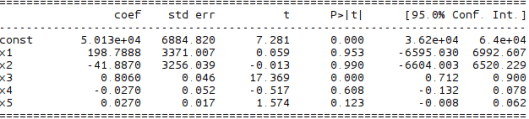
In the image above, x1 and x2 are two dummy variables for the state, x3 is the R&D Spend, x4 is Admin Spend and x5 is Marketing Spend. Now we have to look for the highest P-value which in this case is 0.990 for x2 and according to our algorithm above, we need to remove x2 from the matrix. So let’s do that.
Variable x2 has column index 2 in the matrix x above, so we remove that index and repeat the process by removing indexes from the original matrix with all values.
x_opt = x[:, [0, 1, 3, 4, 5]]
Summary shows that variable x2 with index 2 has the highest significance so we have to remove it from the original matrix. We repeat the process until we reach zeroes in the summary for P-values.
x_opt = x[:, [0, 1, 3, 4, 5]]
regressor_OLS = sm.OLS(endog = y, exog = x_opt).fit()
regressor_OLS.summary()

x_opt = x[:, [0, 3, 4, 5]]
regressor_OLS = sm.OLS(endog = y, exog = x_opt).fit()
regressor_OLS.summary()

x_opt = x[:, [0, 3, 5]]
regressor_OLS = sm.OLS(endog = y, exog = x_opt).fit()
regressor_OLS.summary()

x_opt = x[:, [0, 3]]
regressor_OLS = sm.OLS(endog = y, exog = x_opt).fit()
regressor_OLS.summary()
Here endog means endogenous to our model, which is the dependent variable y, while exog is exogenous to our model which is the independent variable x in our case. In the next posts I will talk about methods which will help us to decide with more certainty which columns to remove.
Resources:
