Support Vector Machine (SVM)

Support Vector Machine is a supervised learning type of algorithm and its goal is to find the optimal hyperplane which separates clusters of data. In 1D we will have a line instead of a hyperplane and in 2D it will be a plane. In higher dimensions only, we call it a hyperplane. Suppose we have a data with some positive and some negative examples. How do we divide positive examples from the negative ones?

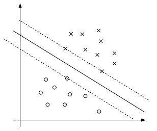
The dataset with two clusters of positive (x) and negative (o) examples. Image is taken from http://cs229.stanford.edu/notes/cs229-notes3.pdf

Vladimir Vapnik suggested drawing a straight line to separate them. This is the simplest linear SVM for linearly separable data (not all data is linearly separable). The question that SVM is trying to answer is – which straight line? There are (infinitely) many possibilities. In the figure above, we have three lines. The middle full line was our first and obvious choice and it is the best one. Our goal is to have the line which leaves as much space as possible from the boundaries. The widest margin we can get in our case is represented by two dotted lines. This is an optimization problem and I will explain the details and mathematics below. Then I will show how to implement it in Python.

Hyperplane is the linear equation of the form

$w_{1}x_{1} +w_{2}x_{2} + \cdots +w_{n}x_{n} = b$

It separates the space into two half-spaces:

$w_{1}x_{1} +w_{2}x_{2} + \cdots +w_{n}x_{n} < b$

and

$w_{1}x_{1} +w_{2}x_{2} + \cdots +w_{n}x_{n} > b$

Hyperplanes are used in many other machine learning algorithms, such as decision trees to define decision boundaries.

We can write the hyperplane formula in the form

$y(x) = \sum_{i=1}^{n}w_{i}x_{i} + b = w^{\tau}x + b \quad (1)$

where vector w is perpendicular to the hyperplane (analogous to the middle full line in the picture above for 2D space) and b is the distance from the origin. We call it the parameters vector or the vector of weights.

In terms of positive and negative samples, formula (1) means that we are taking the dot product of a vector x to the normal vector w, in order to determine whether x belongs to the positive or negative sample (we need to classify it).

Looking at the formula (1) we can see that the middle line equation (which represents the decision boundary) looks like

$w^{\tau}x + b = 0$

Accordingly, if we say that positive and negative samples belong to the set

$y_{i} = \{+1, -1 \}, i = 1, \cdots, n$

then the equations for the support vector lines which represent positive (+1) and negative (-1) examples are given by

$w^{\tau}x + b \geq 1$

$w^{\tau}x + b \leq -1$

If we multiply the equations above with $y_{i}$ , for the middle line we get

$y_{i}(w^{\tau}x_{i} + b) - 1 = 0 \quad (2)$

Now, we want to determine the width between the support vector hyperplanes. We can do that using the dot product between the difference of the two vectors pointing to the support points and the unit vector. This unit vector will be w divided by the magnitude of w. If we mark the vector to the positive sample with $x_{+}$ and the vector to the point that belongs in the negative sample $x_{-}$ , we can write

$\text{width} = (x_{+} -x_{-}) \frac{w}{\|w\|} \quad (3)$

Inserting values from (2) into (3) we get

$(1-b + 1+b) \frac{w}{\|w\|} =\frac{2}{\|w\|} \quad (4)$

which is the length between the two support vector lines and we want to maximize it. So, what we want to do is

$max \frac{2}{\|w\|} \to max \frac{1}{\|w\|}$

or equivalently

$min \frac{1}{2}\|w\|^2$

subject to the vector w. This is a quadratic optimization problem with linear constraints and to solve it we can use Lagrange multipliers. Since it is quadratic, it is convex with a single minimum. This is not the case, for example in neural networks.

In general, we have some function

$f(x_{1}, x_{2}, \cdots, x_{n}) : \mathbb{R}^{n} \to \mathbb{R}$

and we want to optimize f, while contraining it with function g

$g(x_{1}, x_{2}, \cdots, x_{n}) = 0$

The main equation that we use with Lagrangian multipliers is

$\nabla f(x) = \alpha \nabla g(x)$

The Lagrangian function is then

$L(x, \alpha) = f(x) - \alpha g(x)$

Using this equation, we look for points where

$\nabla L(x, \alpha) = 0$

In our case, the Lagrangian function is

$L(w, b, \alpha) = \frac{1}{2} \|w\|^2 - \sum_{i} \alpha_{i} [ y_{i}(w x_{i} + b) - 1 ] \quad (5)$

Taking partial derivatives, we get

$\frac{\partial L}{\partial w} = w - \sum_{i} \alpha_{i} y_{i} x_{i} = 0$

From there follows

$w = \sum_{i} \alpha_{i} y_{i} x_{i}$

Now taking the partial derivative over b,

$\frac{\partial L}{\partial b} = - \sum_{i} \alpha_{i} y_{i} = 0$

This gives us

$\sum_{i} \alpha_{i} y_{i} = 0$

Substituting w back into (5) leads to

$L(w, b, \alpha) = \frac{1}{2} (\sum_{i} \alpha_{i} y_{i} x_{i})(\sum_{j} \alpha_{j} y_{j} x_{j}) - (\sum_{i}\alpha_{i} y_{i} x_{i})(\sum_{j} \alpha_{j} y_{j} x_{j}) - \sum_{i} \alpha_{i} y_{i} + \sum_{i} \alpha_{i}$

Since the second last term equals zero, this becomes

$L(w, b, \alpha) = \sum_{i} \alpha_{i} - \frac{1}{2} \sum_{i}\sum_{j} \alpha_{i}\alpha_{j} y_{i} y_{j} x_{i} \cdot x_{j} \quad (5)$

and this is the formula we want to maximize. We can see that the Lagrangian depends on samples dot product

$x_{i} \cdot x_{j}$

Now substituting the vector w into (2) leads to

$\sum_{i} \alpha_{i} y_{i} \cdot x_{i} + b = 0$

We have a total dependence on the dot products. Dot products tell us how alike features are. If $x_{i}, x_{j}$ are similar, their dot product will be one and they will contribute to the correct answer. If the are not similar, their dot product will be zero and they will not contribute to the answer.

But, what in the case when out data is not linearly separable? In that case, we can take a transformation which will take us from the space we are in, into a different space where we will be able to separate the data. Since maximization depends only on dot products, we can take the transformation of one vector, dotted with the transformation of another vector. The resulting function is called a Kernel function and we define it as

$K(x_{i}, x_{j}) = \phi(x_{i}) \cdot \phi(x_{j})$

where

$\phi(x_{i}), \phi(x_{j})$

are vector transformations. Some commonly used kernel functions are linear, polynomial, and Gaussian kernels. Kernel functions are the reason why the SVM algorithms are so popular. If we have a data that is not linearly separable, we can apply a kernel function to it and transform it into a higher dimension in a way that is not computationally expensive. Then, in this higher dimension, we can linearly separate the data. This is usually called ‘the kernel trick’. Of course, there are constraints in which scenarios this is possible, but I won’t be talking about that now.

Now let’s switch to Python [1]. Suppose we have the following CSV file:

User ID	Gender	Age	EstimatedSalary	Purchased
15624510	Male	19	19000	0
15810944	Male	35	20000	0
15668575	Female	26	43000	0
15603246	Female	27	57000	0
15804002	Male	19	76000	0
15728773	Male	27	58000	0
15598044	Female	27	84000	0
15694829	Female	32	150000	1
15600575	Male	25	33000	0
15727311	Female	35	65000	0
15570769	Female	26	80000	0
15606274	Female	26	52000	0
15746139	Male	20	86000	0
15704987	Male	32	18000	0
15628972	Male	18	82000	0
15697686	Male	29	80000	0
15733883	Male	47	25000	1
15617482	Male	45	26000	1
15704583	Male	46	28000	1

We are trying to predict which users are going to make a purchase (buy the SUV car) according to their salary, gender, and age, and which users are not likely to buy it. As usual, we will first import some utility libraries that we are going to use.

import numpy as np
import matplotlib.pyplot as plt
import pandas as pd

Then we need to import the dataset and split it into the training and test sets. Also, we need to do a feature scaling since the ‘Estimated Salary’ and ‘Age’ columns, for example, have different scales.

dataset = pd.read_csv('social_network_ads.csv')
x = dataset.iloc[:, [2, 3]].values
y = dataset.iloc[:, 4].values

from sklearn.cross_validation import train_test_split
x_train, x_test, y_train, y_test = train_test_split(X, y, test_size = 0.25, random_state = 0)

from sklearn.preprocessing import StandardScaler
sc = StandardScaler()
x_train = sc.fit_transform(x_train)
x_test = sc.transform(x_test)

Now we are ready to start with the SVM. We will import svm library from sklearn and fit svm to the training set, using linear kernel function.

from sklearn.svm import SVC
classifier = SVC(kernel = 'linear', random_state = 0)
classifier.fit(x_train, y_train)

The next step is to predict the test set results.

y_pred = classifier.predict(x_test)

Now, all that is left to do is to visualize results. First, let’s see how the training set looks like.

from matplotlib.colors import ListedColormap
x_set, y_set = x_train, y_train

X1, X2 = np.meshgrid(np.arange(start = X_set[:, 0].min() - 1, stop = X_set[:, 0].max() + 1, step = 0.01),
                     np.arange(start = X_set[:, 1].min() - 1, stop = X_set[:, 1].max() + 1, step = 0.01))

plt.contourf(X1, X2, classifier.predict(np.array([X1.ravel(), X2.ravel()]).T).reshape(X1.shape),
             alpha = 0.75, cmap = ListedColormap(('red', 'green')))
plt.xlim(X1.min(), X1.max())
plt.ylim(X2.min(), X2.max())

for i, j in enumerate(np.unique(y_set)):
  plt.scatter(X_set[y_set == j, 0], X_set[y_set == j, 1],
              c = ListedColormap(('red', 'green'))(i), label = j)
plt.title('SVM (Training set)')
plt.xlabel('Age')
plt.ylabel('Estimated Salary')
plt.legend()
plt.show()

This gives us the following picture

svm-training

Here, points represent what really happened, whether the user purchased the SUV (green points), or not (red points). We also have green and red regions. Any user falling inside the red region is predicted not to buy the SUV, and similarly, any user falling inside the green region is predicted to buy the SUV. The separating curve between the regions is called the prediction boundary.

We can see that predictions could be better. Green points around the point (1, -1) and green points around (-1, 2) ended up incorrectly inside the red region. The reason for this incorrect result is that we have chosen the linear kernel on a data which is not linearly separable.

And finally, the test set results will give us similar predictions.

from matplotlib.colors import ListedColormap
x_set, y_set = x_test, y_test

X1, X2 = np.meshgrid(np.arange(start = X_set[:, 0].min() - 1, stop = X_set[:, 0].max() + 1, step = 0.01),
                     np.arange(start = X_set[:, 1].min() - 1, stop = X_set[:, 1].max() + 1, step = 0.01))
plt.contourf(X1, X2, classifier.predict(np.array([X1.ravel(), X2.ravel()]).T).reshape(X1.shape),
             alpha = 0.75, cmap = ListedColormap(('red', 'green')))
plt.xlim(X1.min(), X1.max())
plt.ylim(X2.min(), X2.max())

for i, j in enumerate(np.unique(y_set)):
  plt.scatter(X_set[y_set == j, 0], X_set[y_set == j, 1],
              c = ListedColormap(('red', 'green'))(i), label = j)
plt.title('SVM (Test set)')
plt.xlabel('Age')
plt.ylabel('Estimated Salary')
plt.legend()
plt.show()

svm-test

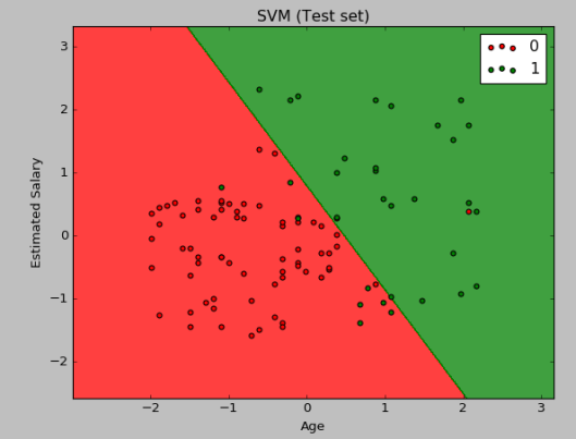
Those predictions are also not so good because the linear kernel is unable to separate the data properly. How can we improve this? We can, of course, try a different kernel function which is more convenient for data which is not linearly separable. We can try this with a Gaussian radial basis function kernel (RBF)

$K(x, x^{\prime}) = exp(- \frac{\|x - x^{\prime}\|^2}{2 \sigma^2})$

where

$x, x^{\prime}$

are feature vectors and $\sigma$ is a free parameter.

The only thing that we need to change in our code above is the SVM classifier part. So, instead of a ‘linear’ function, we will use the ‘rbf’ function.

from sklearn.svm import SVC
classifier = SVC(kernel = 'rbf', random_state = 0)
classifier.fit(x_train, y_train)

Visualization for the training set gives

svm-kernel-training

We can see that this is much better than in the case of the linear kernel function. Some of the green points in the middle are still inside the red region but that is still good because the SVM kernel is not overfitting data.

For more information about this broad topic, please use the comment section or see resources below.

Resources:

Coffee and PI

~ Mathematics. Machine Learning. Data Science.

Support Vector Machine (SVM)

Leave a comment Cancel reply

Share this:

Leave a comment Cancel reply