Imagine you are working at a major investment bank like J.P. Morgan or Goldman Sachs, or maybe at a hedge fund, where modeling how the market behaves is critical, whether for trading strategies, risk controls, or stress scenario simulations. In these types of environments, being able to generate realistic synthetic financial time-series data isn’t just a nice-to-have – it is necessary.

Financial market data is messy: it’s high-dimensional, noisy, non-stationary, and full of seasonality and calendar effects (like month-end anomalies). Classic forecasting models often fall short here, especially when faced with outliers or structural changes in behavior.

To tackle this, I built a generative model – a GAN-based architecture specifically designed for financial time-series data:

• The generator is a Transformer that learns to generate the next day’s features from a short rolling window of previous days.
• The discriminator is a feedforward network that tries to tell apart real vs. generated next-day data.
• The generator loss blends Binary Cross Entropy, MSE, and a custom volume-aware term to better handle the scale mismatch between price and volume.
• A Gaussian noise layer is added to the generator, which helps avoid mode collapse and encourages more diverse outputs.
• Ticker (stock name) embeddings to let the model generalize across multiple stocks while still capturing their unique behaviors.

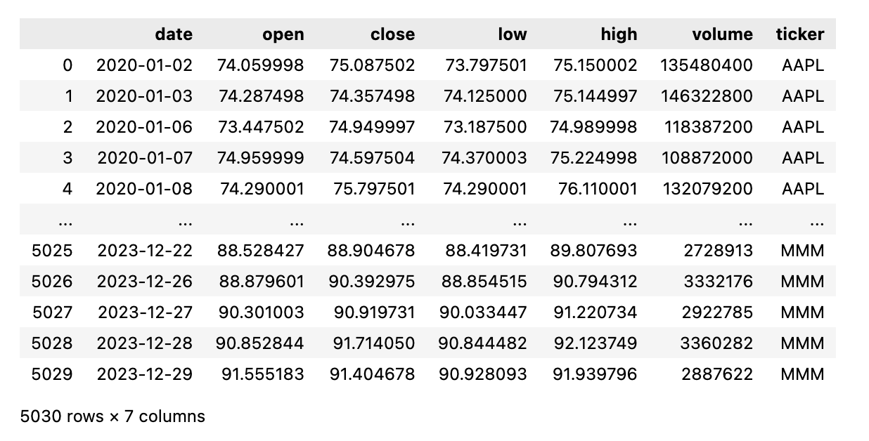
I got three years of trading data from Yahoo Finance (2020 – 2023) for stocks (tickers) Apple, Microsoft, Amazon, Google, and 3M, which I downloaded using yfinance (https://pypi.org/project/yfinance/) library in Python.

It consists of:

• OHLC Features: Open, High, Low, Close
• Volume Feature
• Date Feature
• Ticker Name Feature

First, I split the data into time series train, validation, and test sets.

train_data, val_data, test_data = split_time_series(data)

assert val_data.date.min() > train_data.date.max()
assert test_data.date.min() > val_data.date.max()

INFO – Data split sizes – Train: 3520, Val: 755, Test: 755

Training Data Distribution:
ticker
AAPL     704
MSFT     704
AMZN     704
GOOGL    704
MMM      704
Total training samples: 3520

Validation Data Distribution:
ticker
AAPL     151
MSFT     151
AMZN     151
GOOGL    151
MMM      151
Total validation samples: 755

Test Data Distribution:
ticker
AAPL     151
MSFT     151
AMZN     151
GOOGL    151
MMM      151
Total test samples: 755

Training period: 2020-01-02 00:00:00 to 2022-10-17 00:00:00
Validation period: 2022-10-18 00:00:00 to 2023-05-24 00:00:00
Test period: 2023-05-25 00:00:00 to 2023-12-29 00:00:00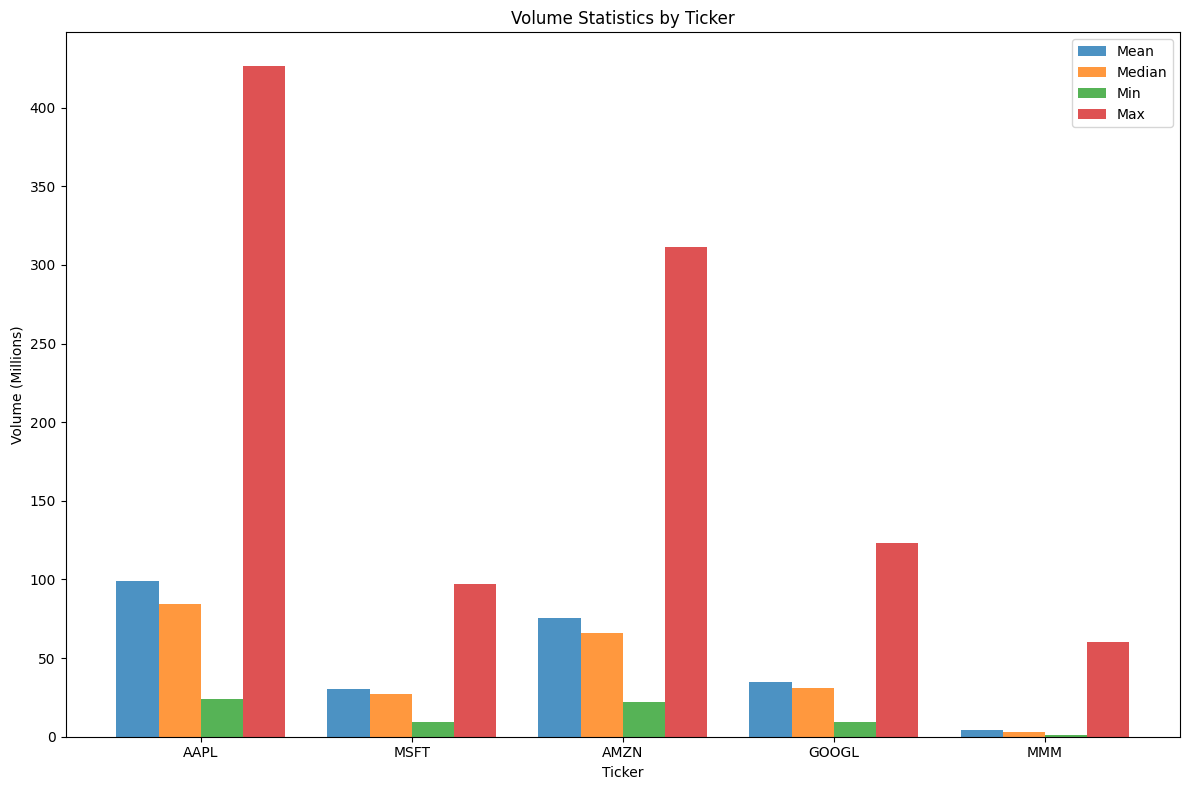

We can see that volume differs across tickers. This will be important for training and incorporating volume-aware loss.

I am generating synthetic data here based on existing data and tickers, so I presume that all tickers will be seen in inference time.

Feature Generation

I created new cyclic features from the date column by using sin and cos of “day”, “month”, “quarter”. Each of them has 2 features – sin and cos versions (so 6 features in total).

    if cyclic_config['day']:
        df['day'] = df['date'].dt.dayofweek
        features.extend([
            np.sin(2 * np.pi * df['day'] / 7),
            np.cos(2 * np.pi * df['day'] / 7)
        ])

The input model size is:

input_size = 4 OHLC features + 1 volume feature + 6 cyclic features = 11  features

Let’s have a look at the Amazon ticker example of how original vs. normalized data looks. Each ticker is normalized independently to account for varying price/volume scales across instruments.

OHLC Normalization: Raw Prices vs Returns

For this project, I normalize price features in the followig way:

        # OHLC normalization
        data_ohlc = df_filtered.iloc[:, 1:5].values
        ohlc_scaler = RobustScaler()
        norm_ohlc = ohlc_scaler.fit_transform(data_ohlc)

Alternative approach: I used raw prices, but you could also use returns (df.pct_change()) instead of raw prices. Returns are more stationary and often better for time series modeling, but raw prices preserve the absolute relationships needed for certain financial applications.

Volume Normalization

Volume data presents three distinct challenges: extreme skewness, temporal regime changes, and inconsistent ranges, as we can see from the plot above. I address these with a three-stage normalization process:

• Step 1 – Log1p Transform: Volume data is heavily right-skewed. The log transformation stabilizes variance and makes the distribution more Gaussian-like.
• Step 2 – Rolling Z-Score: Financial markets exhibit changes where volume shifts dramatically. Rolling statistics capture temporal context, i.e., what is unusual for this period only, rather than historically.
• Step 3 – Robust Range Control: Even after log transformation and rolling normalization, we need consistent feature ranges for stable GAN training. RobustScaler provides data-driven bounds without arbitrary clipping.

As seen in the normalized plot above, the result is a roughly uniform spread of values, which helps when training neural networks. This is especially important in GANs, where stable training requires input features to be both centered and consistent over time.

        # Volume normalization
        data_volume = df_filtered['volume'].values.reshape(-1, 1)
        volume_transformed = np.log1p(data_volume)

        # Calculate rolling statistics
        volume_series = pd.Series(volume_transformed.ravel())
        volume_mean = volume_series.rolling(window=rolling_window, min_periods=1).mean()
        volume_std = volume_series.rolling(window=rolling_window, min_periods=1).std()

        # Fill NaN values
        volume_mean = volume_mean.bfill()
        volume_std = volume_std.bfill().fillna(volume_std.mean())
        volume_relative = ((volume_transformed.ravel() - volume_mean.to_numpy()) /
                         (volume_std.to_numpy() + 1e-8))

        volume_scaler = RobustScaler(quantile_range=(10, 90))
        norm_volume = volume_scaler.fit_transform(
            volume_relative.reshape(-1, 1)
        ).ravel()

To train a model on time-series data, I first transformed each ticker’s historical records into sequences. A sequence is a short window of consecutive days – for example, 10 days of OHLC, volume, and date features. Each sequence captures a small piece of the stock’s timeline.

I used sequence_length = 10, for which the transformation creates overlapping windows:

Historical Data Timeline:
Day 1: [OHLC + volume + date features]  ← 11 total features
Day 2: [OHLC + volume + date features]
Day 3: [OHLC + volume + date features]
...
Day 10: [OHLC + volume + date features]
Day 11: [OHLC + volume + date features]
Day 12: [OHLC + volume + date features]
...

Generated Training Sequences:
Sequence 1: Days 1→10 predict Day 11
Sequence 2: Days 2→11 predict Day 12  
Sequence 3: Days 3→12 predict Day 13
...

I created sequences from stacked OHLC, volume, and dates data:

combined_data = np.hstack([
            data['norm_ohlc'],
            data['norm_volume'].reshape(-1, 1),
            data['cyclic_dates']
        ])

Why This Approach?

When you have, say, 1000 trading days of history, you can create around 995 overlapping training sequences instead of just using the data once. This means the model sees way more examples of how markets behave in different situations.

More importantly, each sequence gives the model recent context to work with. Financial markets aren’t random – if there was a big earnings announcement 3 days ago or unusual volume yesterday, that matters for predicting tomorrow. The model learns to pick up on these short-term patterns that actually persist across different stocks and market conditions.

Why 10 Days Specifically?

Ten days is roughly two business weeks, which captures short-term momentum while including those weekly patterns you see in markets, like how Mondays often behave differently after weekend news, or how volume tends to pick up toward the weekend.

From a practical standpoint, 10 days gives the transformer enough context to spot meaningful patterns without drowning it in too much history. Markets have momentum, and this approach captures that temporal flow rather than treating each day in isolation. I would like to experiment with this further.

Generator

My generator uses a Transformer encoder architecture for sequence-to-point prediction. Unlike RNNs that process sequences step-by-step, transformers can “look at” all previous days simultaneously through attention mechanisms, capturing temporal relationships in financial markets.

"""
Generator module implementing a Transformer-based architecture for synthetic financial data generation.
"""

class TransformerGenerator(nn.Module):
    """
    Transformer-based generator for financial time series data.
    
    Uses a transformer encoder architecture to generate synthetic financial data,
    processing OHLC prices, volume, and cyclic date features.
    """

    def __init__(
        self,
        input_size: int,
        num_layers: int,
        d_model: int,
        nhead: int,
        dim_feedforward: int,
        output_size: int,
        dropout: float,
        num_tickers: int,
        ticker_embedding_dim: int,
        noise_dim: int = 8
    ) -> None:
        """
        Initialize the generator.

        Args:
            input_size: Number of input features (OHLC + volume + enabled cyclic features)
            num_layers: Number of transformer encoder layers
            d_model: Dimension of the transformer model
            nhead: Number of attention heads
            dim_feedforward: Dimension of feedforward network in transformer
            output_size: Number of output features (same as input_size)
            dropout: Dropout rate for regularization
        """
        super().__init__()
        self.noise_dim = noise_dim
        self.noise_projection = nn.Linear(noise_dim, d_model)
        
        self.input_size = input_size
        self.embedding_dim = ticker_embedding_dim
        self.ticker_embedding = nn.Embedding(num_tickers, ticker_embedding_dim)

        self.positional_encoding = nn.Linear(input_size + ticker_embedding_dim, d_model)
        self.price_linear = nn.Linear(d_model, d_model)

        encoder_layer = nn.TransformerEncoderLayer(
            d_model=d_model,
            nhead=nhead,
            dim_feedforward=dim_feedforward,
            dropout=dropout,
            batch_first=True
        )

        self.transformer_encoder = nn.TransformerEncoder(
            encoder_layer, 
            num_layers=num_layers
        )

        self.feature_decoder = nn.Sequential(
            nn.Linear(d_model, d_model),
            nn.ReLU(),
            nn.Dropout(dropout),
            nn.Linear(d_model, output_size)
        )

        self.norm1 = nn.LayerNorm(d_model)
        self.norm2 = nn.LayerNorm(d_model)
    
    def forward(
        self,
        src: torch.Tensor, 
        ticker_idx: torch.Tensor,
        noise: Optional[torch.Tensor] = None
    ) -> torch.Tensor:

        embed = self.ticker_embedding(ticker_idx).unsqueeze(1).repeat(1, src.shape[1], 1)
        x = torch.cat([src, embed], dim=-1)
        x = self.positional_encoding(x)
        x = self.norm1(x)

        if noise is None:
            noise = torch.randn(src.size(0), self.noise_dim, device=src.device)

        noise_proj = self.noise_projection(noise)  # Shape: (batch_size, d_model)
        noise_proj = noise_proj.unsqueeze(1).repeat(1, src.size(1), 1)
        x = x + noise_proj

        price_features = self.price_linear(x)
        x = x + price_features
        x = self.norm2(x)

        output = self.transformer_encoder(x)
        output = self.feature_decoder(output[:, -1, :])
        output = self._apply_financial_constraints(output)
        return output


    def _apply_financial_constraints(self, output: torch.Tensor) -> torch.Tensor:
        """
        Apply financial constraints to generator output.
        
        Args:
            output: Raw generator output of shape (batch_size, output_size)
            
        Returns:
            Constrained output respecting financial relationships
        """
        # Split output into components
        open_price = output[:, 0:1]   # Open
        high_price = output[:, 1:2]   # High
        low_price = output[:, 2:3]    # Low
        close_price = output[:, 3:4]  # Close
        volume = torch.relu(output[:, 4:5])  # Volume must be positive
        
        if output.size(1) > 5:  # If we have cyclic features
            cyclic_features = output[:, 5:]
        else:
            cyclic_features = torch.empty(output.size(0), 0, device=output.device)

        # Apply OHLC constraints
        constrained_ohlc = self._enforce_ohlc_constraints(open_price, high_price, low_price, close_price)

        return torch.cat([constrained_ohlc, volume, cyclic_features], dim=1)

    def _enforce_ohlc_constraints(self, open_p: torch.Tensor, high_p: torch.Tensor,
                                 low_p: torch.Tensor, close_p: torch.Tensor) -> torch.Tensor:
        """
        Enforce OHLC financial constraints:
        - High >= max(Open, Close)
        - Low <= min(Open, Close)
        
        Args:
            open_p, high_p, low_p, close_p: Individual OHLC price tensors
            
        Returns:
            Constrained OHLC tensor of shape (batch_size, 4)
        """
        # High >= max(Open, Close)
        min_high = torch.max(open_p, close_p)
        constrained_high = torch.max(high_p, min_high)

        # Low <= min(Open, Close)  
        max_low = torch.min(open_p, close_p)
        constrained_low = torch.min(low_p, max_low)

        return torch.cat([open_p, constrained_high, constrained_low, close_p], dim=1)

Financial Constraints: I enforced financial relationships, making sure that High ≥ max(Open, Close), Low ≤ min(Open, Close), and positive volume. This prevents the generation of financially impossible data while maintaining learned patterns.

Discriminator

While the generator needs to understand temporal sequences, the discriminator has a simpler job: given OHLC, volume, and date features for one day, it determines if the data looks real or generated.

class Discriminator(nn.Module):
    """
    Discriminator network for GAN architecture.

    Processes financial data including OHLC, volume, and cyclic features to
    determine if the input is real or generated. Architecture consists of
    fully connected layers with batch normalization, LeakyReLU,
    and dropout, ending with a sigmoid activation for binary classification.
    """

    def __init__(
        self,
        input_size: int,
        hidden_sizes: List[int],
        dropout: float,
        leaky_relu_slope: float
    ) -> None:
        """
        Initialize the discriminator.

        Args:
            input_size: Number of input features (OHLC + volume + enabled cyclic features)
            hidden_sizes: List of sizes for hidden layers
            dropout: Dropout rate for regularization
            leaky_relu_slope: Negative slope coefficient for LeakyReLU activation
        """
        super().__init__()

        layers = []
        current_size = input_size

        for hidden_size in hidden_sizes:
            layers.extend([
                nn.Linear(current_size, hidden_size),
                nn.BatchNorm1d(hidden_size),
                nn.LeakyReLU(leaky_relu_slope),
                nn.Dropout(dropout)
            ])
            current_size = hidden_size

        layers.extend([
            nn.Linear(hidden_sizes[-1], 1),
            nn.Sigmoid()
        ])

        self.model = nn.Sequential(*layers)

    def forward(self, x: torch.Tensor) -> torch.Tensor:
        """
        Forward pass of the discriminator.

        Args:
            x: Input tensor of shape (batch_size, input_size) containing
               normalized financial data features

        Returns:
            Tensor of shape (batch_size, 1) containing probabilities
            that each input sample is real (1) vs generated (0)
        """
        return self.model(x)

A feedforward network with batch normalization and dropout handles this classification task. This architectural choice reflects the different nature of each model’s task – sequence understanding vs. point classification.

Why Point Prediction for Synthetic Data Generation

I chose single-step (point) prediction over multi-step sequence prediction for several reasons:

Point prediction is significantly more stable to train. The model learns one objective – to predict tomorrow given the last 10 days – rather than juggling multiple future time steps with increasing uncertainty. By applying the model iteratively, I can generate sequences of any length (10 days, 100 days, or 1000 days) without architectural changes. Also, with point prediction, errors accumulate naturally through iteration, mimicking real market dynamics. Sequence prediction can compound errors within the model itself, leading to unrealistic long-term behavior.

Information Bottleneck Problem: RNNs compress all historical information through a fixed-dimensional hidden state, causing critical market events (like earnings from 2 weeks ago) to decay exponentially. Transformers solve this with direct attention – every day can directly “look at” any previous day, enabling the model to recognize that day t-10 might be more relevant than day t-1 for predicting today’s price.

Multi-Head Specialization: I used 2 attention heads, which gives the model the capacity to potentially specialize in different aspects of the financial data. In theory, one might focus more on price dynamics while another captures volume patterns, but the actual specialization emerges during training and would require attention-weight analysis to verify.

Mathematical Foundation: The attention mechanism

The attention weights are

representing how much day i “pays attention to” day j when making predictions.

My hybrid loss balances two key objectives:

Volume-Aware Loss: Scales the MSE for volume depending on the stock’s typical trading volume, ensuring smaller-volume tickers aren’t ignored.

Adversarial Realism – Ensuring that the generated data is indistinguishable from real financial data via Binary Cross Entropy (BCE).

Reconstruction Accuracy – Using a composite MSE loss, which itself consists of:

• Regular MSE: Penalizes deviations in OHLC and cyclic features.
• Volume-Aware Loss: Scales the MSE for volume depending on the stock’s typical trading volume, ensuring smaller-volume tickers aren’t ignored.

            g_loss_adv = adversarial_loss(fake_outputs, real_labels)

            volume_feature_idx = 4  # Volume is the 5th feature (index 4)

            # Regular MSE for OHLC and cyclic features
            non_volume_features = torch.cat([
                fake_data[:, :volume_feature_idx],      # OHLC features (0-3)
                fake_data[:, volume_feature_idx+1:]     # Cyclic features (5+)
            ], dim=1)

            non_volume_targets = torch.cat([
                batch_y[:, :volume_feature_idx],
                batch_y[:, volume_feature_idx+1:]
            ], dim=1)
            
            # Regular MSE loss: penalizes errors in OHLC and cyclic date features
            g_loss_regular = mse_loss(non_volume_features, non_volume_targets)
            
            # Volume-aware loss for volume feature
            g_loss_volume = volume_aware_loss(
                fake_data[:, volume_feature_idx], 
                batch_y[:, volume_feature_idx],
                batch_vol_weights,
                device
            )

            # Combine losses
            g_loss_mse = g_loss_regular + g_loss_volume
            adv_weight = config['training_params']['adv_weight']
            g_loss = adv_weight * g_loss_adv + (1 - adv_weight) * g_loss_mse

and with adv_weight = 0.5, this becomes:

Why 50-50 Split? This came from experimentation, but more testing is necessary.

Combined loss: The adversarial part makes sure the generated data looks like real market data statistically. MSE part keeps the predictions accurate and prevents the model from going completely off the rails, whilst volume weighting stops AAPL’s huge volume (~57M daily), for example, from drowning out MMM’s smaller volume (~4.5M) during training. Because of this difference in volume across stocks, after I added volume-aware loss, the error improved by 20%.

The adversarial term maximizes Jensen-Shannon divergence for distributional matching, while MSE provides L2 regularization for local continuity.

I used the following architecture (for the full details, see the config.json file):

Generator (Transformer):

• Layers: 2 transformer encoder layers
• Model Dimension: 64 (d_model)
• Attention Heads: 2
• Feedforward Dimension: 128
• Dropout: 0.1

Discriminator (Feedforward):

• Hidden Layers: [128, 64] neurons
• Activation: LeakyReLU (slope=0.2)
• Dropout: 0.1
• Output: Single probability (real vs. fake)

Training Configuration:

• Sequence Length: 10 days
• Batch Size: 64
• Epochs: 100 (with early stopping)
• Learning Rate: 0.001 (both G and D)
• Combined Loss: 50% adversarial + 50% MSE
• Warmup: 5 epochs

Training Results

The training loop follows a standard adversarial GAN setup, where the generator and discriminator are trained in tandem. For the generator, I apply the hybrid loss function described above, balancing adversarial realism with reconstruction accuracy.

After 17 epochs of training with early stopping, the model achieved convergence:

Learning Rate Scheduling

• Epochs 1–5: Warmup phase – LR increased gradually from 0.0002 → 0.001
• Epochs 6–11: Full learning rate maintained (0.001)
• Epoch 12: LR reduced to 0.0005 after validation plateau
• Epoch 16: LR reduced further to 0.00025
• Early Stopping: Triggered at epoch 17

Validation Loss Performance

• Initial loss (epoch 1): 0.5515
• Best performance: 0.1950 (achieved at epoch 8)
• Final computed loss (epoch 18): 0.2710

Training remained stable, especially during the warmup phase, with the generator and discriminator improving in tandem. Early stopping was triggered at epoch 17, just after the second scheduled learning rate decay, following a plateau in validation loss.

Cross-Ticker Training Strategy + Conditional Modeling

Rather than train a separate model for each stock, I pooled all tickers together and used per-ticker normalization to align distributions. To preserve each ticker’s identity while enabling cross-ticker generalization, I introduced the following:

• Learned Ticker Embeddings: Instead of one-hot vectors, each ticker is represented as a trainable embedding vector, enabling the model to learn latent ticker-specific behavior. These embeddings are passed into the generator alongside price/volume sequences.
• Gaussian Noise Injection: A stochastic noise vector is added inside the generator, just before the decoder. This encourages the model to produce varied yet realistic outputs, avoiding mode collapse or overfitting to deterministic patterns.

Model Design Principles

• Transformer-based Generator: Ideal for capturing financial time-series dynamics like volatility clustering, seasonal effects, and calendar structure.
• Composite Loss Function: A mix of adversarial (BCE), reconstruction (MSE), and volume-aware loss terms ensures that generated sequences are both statistically accurate and financially plausible.
• Volume Normalization: Done in three stages to stabilize training and handle scale differences across tickers.
• Hard Financial Constraints: Enforced (e.g. low ≤ open/close ≤ high) to maintain realism and prevent invalid sequences.
• Early stopping: Caught overfitting at epoch 17 and preserved the best model

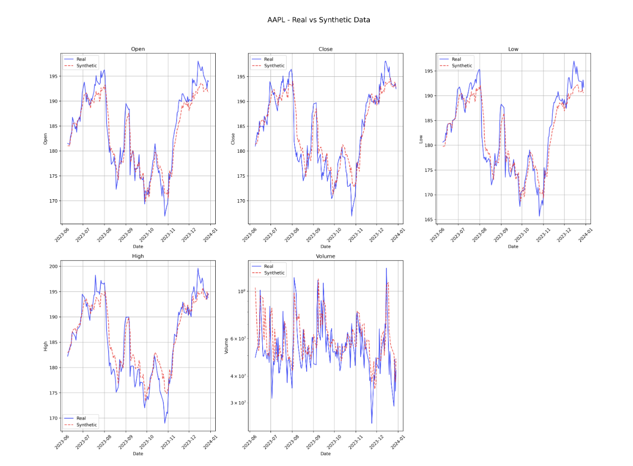
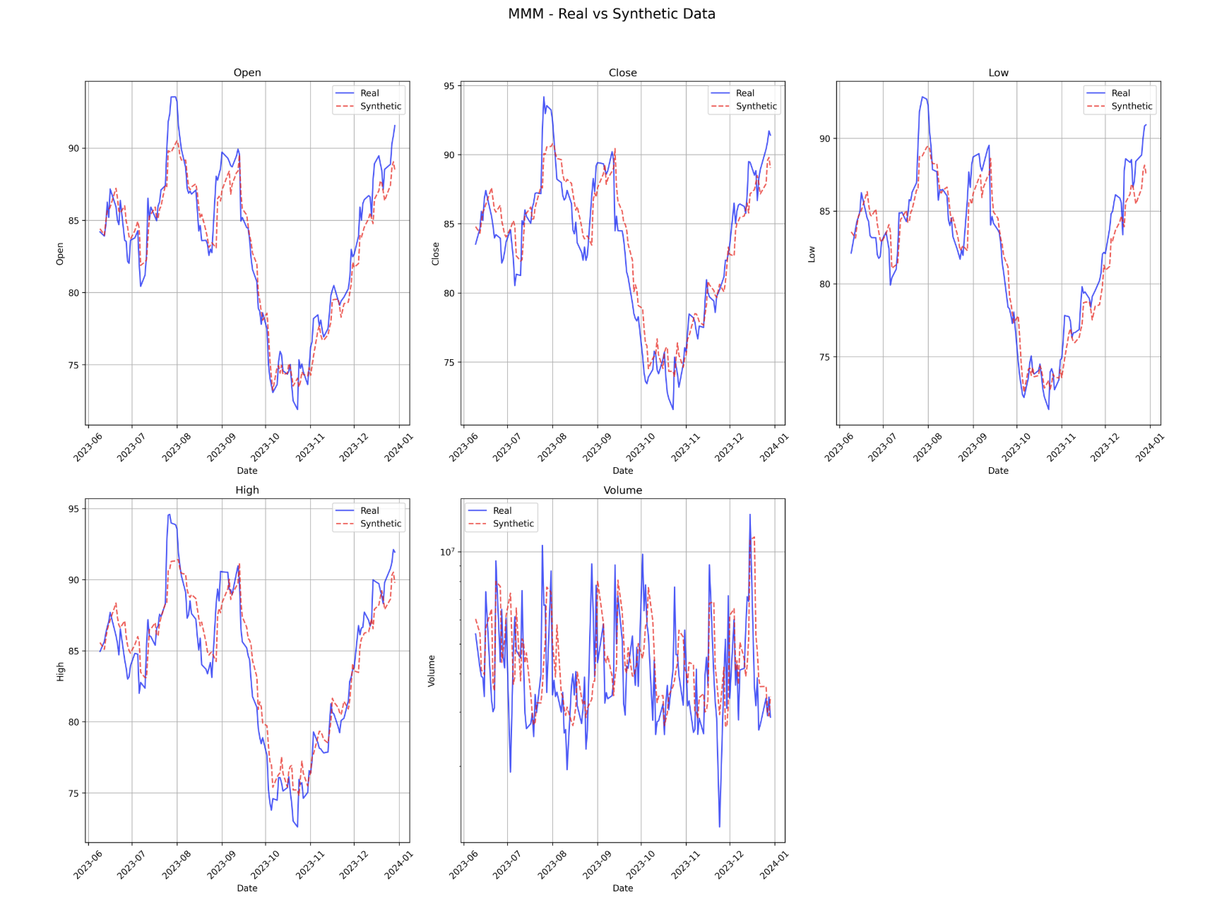
Generated Synthetic Data Examples

Metrics Used

• MAE (Mean Absolute Error): Average absolute difference between predicted and real values. Lower = better. Moderately sensitive to outliers.
• MAPE (Mean Absolute Percentage Error): Percentage-based error, scale-independent. <5% = excellent, <10% = good. Less sensitive to outliers than MAE.
• Correlation: Linear relationship strength (-1 to 1). >0.9 = excellent, >0.7 = good. Sensitive to outliers.
• KL Divergence: How different the generated distribution is from the real (0 = identical, higher = more different). Very sensitive to outliers.
• JS Divergence: Symmetric version of KL (0-1 scale, 0 = identical). Moderately sensitive to outliers.
• Wasserstein Distance (Low Wasserstein = High Quality): “Earth mover’s distance” between distributions. Wasserstein measures the “minimum effort” needed to transform the generated distribution into the real distribution. Robust to outliers.

Each metric captures different aspects – correlation shows relationship strength, MAPE shows prediction accuracy and distribution metrics ensure realistic data generation patterns. Using multiple metrics provides a comprehensive evaluation and guards against metric-specific biases.

Volume Generation – Challenging but Reasonable

Generating realistic volume data remains one of the harder tasks in financial time-series modeling. Unlike prices, volume is highly irregular, less autocorrelated, and often impacted by external news, earnings, or macroeconomic factors.

Results were promising, but further control and incorporation for rare events is necessary:

• Correlation with real data: Ranged between 0.46 and 0.59 across tickers – not perfect, but statistically meaningful, and within what is considered acceptable error in finance for volume.
• MAPE (Mean Absolute Percentage Error): Varied between 20% and 32%, reflecting the naturally high variance and spikes in real-world trading activity.
• KL & JS Divergences: Reasonable across the board – indicating the model captures distributional characteristics.
• Wasserstein Distance: It is big because of spikes in volume, but this is expected due to big spikes in volume. More work on the loss function is needed to minimise this, but other metrics and visual results show that the synthetic data is following closely the distribution of the original data.

Key Improvements:

• Volume-Aware Loss: Explicitly penalizes unrealistic volume behavior and helps the generator prioritize volume learning alongside price accuracy. Adding this improved errors by 20%.
• Ticker Embeddings + Noise: Add diversity and flexibility, allowing the model to learn ticker-specific volume styles and prevent overfitting (e.g., AMZN vs. MMM).

While there’s room to improve, especially for extreme volume spikes or regime shifts, the model’s current volume generation is good enough to support synthetic backtesting and modeling use cases without major distortions.

Volume Analysis Summary:
==================================================
AAPL: Mean=56.7M, MAE=10.5M (18.5% relative)
MSFT: Mean=25.8M, MAE=5.6M (21.9% relative)
AMZN: Mean=53.7M, MAE=10.5M (19.6% relative)
GOOGL: Mean=29.3M, MAE=6.7M (22.8% relative)
MMM: Mean=4.5M, MAE=1.3M (30.0% relative)

Highest volume: AAPL (56.7M)
Lowest volume: MMM (4.5M)
Best MAPE: AAPL (19.8%)
Worst MAPE: MMM (31.9%)

• 19.8% to 31.9% MAPE, reflecting volume’s inherent volatility and noise
  • Low / Close Prices: 1.16% to 2.08% MAPE
  • Performance was boosted by volume-aware loss, although this remains the most difficult feature to synthesize

def volume_aware_loss(pred_volume, real_volume, volume_weights, device):
    """
    Apply volume-scale aware weighting to balance training across different volume regimes
    
    Args:
        pred_volume: Predicted volume values for current batch
        real_volume: Real volume values for current batch  
        volume_weights: Pre-computed volume weights per sample
        device: Training device
    """
    base_loss = nn.MSELoss(reduction='none')(pred_volume, real_volume)

    # Apply volume weighting
    weighted_loss = base_loss * volume_weights.to(device)

    return torch.mean(weighted_loss)

Price Generation (OHLC)

Price generation performance was consistently strong across all tickers and OHLC features:

• Correlation with real prices: Ranged from 0.93 to 0.97, indicating that the generator closely follows the structure of real market movements and captures temporal dependencies.
• MAPE (Mean Absolute Percentage Error): Stayed below 2.1% across all OHLC components — meaning day-to-day generated prices are very close to real ones in absolute terms.
• KL Divergence: Mostly between 0.87 and 2.27, well below typical thresholds, indicating the generated price distributions align well with real data, both in mean and shape.
• Wasserstein Distance & JS Divergence: Remained low, especially for price features, suggesting statistical realism without overfitting or memorization.

• Open Prices: Best performance — 1.03% to 1.99% MAPE
• High Prices: 1.16% to 1.64% MAPE

• I would like to try more sophisticated enforcement of financial relationships between features like intraday volatility bounds, based on historical patterns, for example
• I want to train on more epochs (50+), with more advanced scheduling strategies to push performance further
• Also, use more data and tickers (stocks), currently I am using 5 tickers only across 3 years
• Use longer sequences, monthly or quarterly patterns, with 30-60 day context windows
• Check if synthetic data works well for training other ML models
• Add more unit tests for the codebase itself
• Test distributed training
• Add differential privacy

This project demonstrates that transformer-based GANs can generate synthetic financial data with strong empirical performance, particularly on price features, while also handling challenges such as volume volatility and cross-ticker dynamics.

This is a personal research project, and I am actively testing and improving it.

You can find the code for this project on my GitHub profile – https://github.com/LucijaGregov/financial_synthetic_data_gan_transformer.